If you do not have Microsoft Excel, you can use the XLOOKUP in Google Sheets to manage larger data sheets and enhance your data handling processes.
If we compare HLOOKUP and VLOOKUP with XLOOKUP in Excel, then XLOOKUP is a more flexible and powerful tool to find values.
Here is a quick overview of using the XLKOOKUP in Google Sheets to streamline your data management process.
Note: We’ve just covered some basic steps for using the XLOOKUP in Google Sheets. If you want to know more about XLOOKUP(), such as VLOOKUP() vs XLOOKUP(), why we should use it, what its benefits are, and how Google Sheet XLOOKUP functions, check out our XLOOKUP() Excel page. As you know, this function is the same in both sheets, thus, you can find the details here.
What is XLOOKUP() in Google Sheets? Learn XLOOKUP Step-by-Step
XLOOKUP() is the same as XLOOKUP() in Excel sheets. You can use XLOOKUP in Google Sheets to search or look up a value from a set of data collection. XLOOKUP compares and returns the exact match values, and it may also return the proper match or the last or first matching value, depending on the formula inputs.
Unlike other VLOOKUP() functions, XLOOKUP() returns values horizontally and vertically, and you can retrieve a full row of data rather than just one value.
Syntax: = XLOOKUP(lookup_value, lookup_array, return_array, [if_not_found], [match_mode], [search_mode])- lookup_value: The value we are looking for.
- lookup_array: This is the range or array of columns and rows in which Excel will search for our lookup_value.
- return_array: This will be the range or array of columns and rows from which Excel will return the matching value.
- [if_not_found] (Optional): This will be the message or any value that will be returned if xlookup found no matching value..
- [match_mode] (Optional): This mode will specify the type of match, like whether you are looking for an Exact, Approximate, or Wildcard match.
1. XLOOKUP in Google Sheet: Basic Exact Match
Let’s assume that you are a manager of a store and you need to find the price of a product based on its name using XLOOKUP.
And a customer asks for the price of a Smartwatch. Instead of searching manually, you can use the XLOOKUP formula.
=XLOOKUP(E2, A2:A7, C2:C7)- First, make another column of search key and results, and then add the name of the product that you are looking for in the search key column.
- Now, enter the formula in the results column right after the product name.
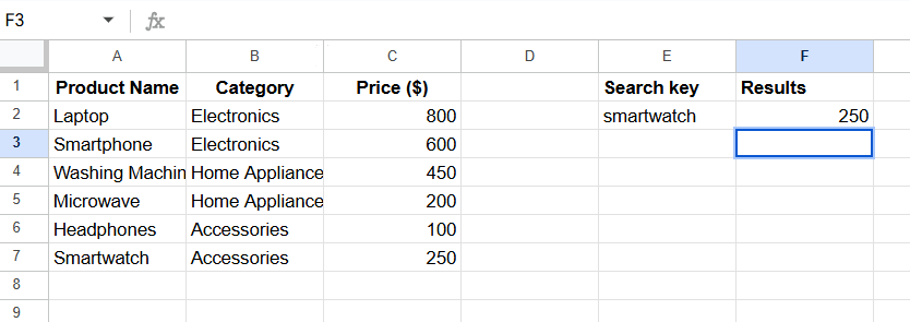
As you can see in the image, the e XLOOKUP() has returned the value based on the product name.
Formula’s Breakdown:
- E2: The cell where you enter the product name (e.g., “Smartwatch”)
- A2:A7: The lookup range (Column A, where product names are listed)
- C2:C7: The return range (Column C, where prices are stored)
2. Product Not Found- Missing Value
And if you don’t find the product in the datasheet, then it will display a #N/A error. To overcome this problem, you can use this formula:
=XLOOKUP(E3, A2:A7, C2:C7, "Product Not Found")
Now you can see that when we enter an irrelevant product, it returns “Product Not Found” instead of a #N/A error.
3. Left XLOOKUP()
VLOOKUP cannot look up for a value to its left; it can only search for a value to the right of the lookup column. But XLOOKUP allows us to search in any direction, including looking to the left.
Example:
Let’s take the previous example and assume that you have to find out which category a product belongs to by searching for its price.
Normally, VLOOKUP requires the lookup column (Price) to be to the left of the return column (Category), which is not the case here. But with XLOOKUP, you can still perform this search without rearranging the table.
To find the category based on the price, you can use this formula:
=XLOOKUP(E3, C2:C7, A2:A7, "Category Not Found")
As you can see in the image, it returns the category based on the price.
If it doesn’t find the category you are looking for, then it will return “Category Not Found” instead of a #N/A error.
4. XLOOKUP() Approximate Match
The 5th mode of the XLOOKUP() function is the matching mode. In this mode, setting it to 0 will return the exact match value. However, there are times when we cannot find an exact match but want an approximate match, such as a number that is higher or lower than the one we are looking for. So, in this case, the approximate match function is really useful.
For Nearest Lowest Value:
Let’s take an example:
You, as a school teacher, want to assign grades to students based on their exam scores. However, students may receive different scores that are not listed exactly in the grading table.
To solve this, you can use XLOOKUP with an approximate match (-1) so that if a student’s score does not exactly match, the function returns the closest lower grade boundary instead.
Now, let’s say a student scores 77 marks in the exam, but 77 is not in the table. And you need to find the nearest lower value (which is 70) and return its corresponding grade.
You can use this formula:
=XLOOKUP(E2, A2:A6, B2:B6, "Fail", -1)
As you can see in the image, it has returned grades for the nearest lowest value of 77.
The 4th argument in the formula mentioned that if the student’s score is below 50, they will be marked as “Fail”
For Nearest Highest Value:
If the exact match is not found and you want the output as the nearest highest value, then you can replace 1 with -1 in the formula.
=XLOOKUP(E3, A2:A6, B2:B6, "Fail", 1)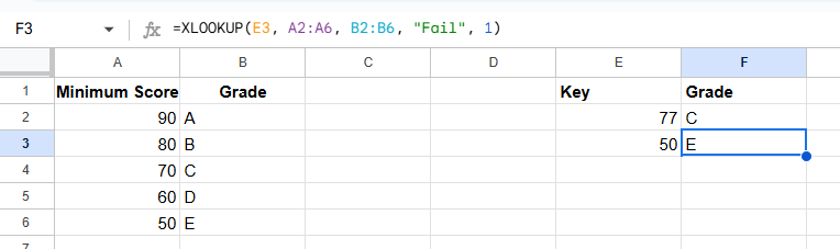
5. XLOOKUP() Wildcard Match
Google sheet XLOOKUP() supports three wildcards: *,?, and ~.
The asterisk (*) represents any number of characters (including none).
- Example: Searching for “Ba*” would match “Banana”, “Ball”, and “Basket”.
The question mark (?) represents exactly one character in a string.
- Example: Searching for “A?C” would match “ABC”, and “ACC”, but not “AC” or “ABBC”.
The tilde (~) is an escape character, used when you want to search for a literal * or? Instead of treating them as wildcards.
- Example: Searching for “File~*” would find “File*” (with an actual asterisk), not words starting with “File”.
Example: Using * (Asterisk)
Let’s say that you have a list of employees and their departments. You want to find employees based on partial names.
You want to find the department of an employee whose name starts with “A”. You can use this formula:
=XLOOKUP("A*", A2:A6, B2:B6, "Not Found", 2)
As you can see, it returns “HR” because Alice Johnson matches “A”.
XLOOKUP in Google Sheets does not support the? Wildcard directly for single-character matching as it does with *. Instead, we need to use the FILTER or SEARCH functions for such cases.
6. Google Sheet XLOOKUP(): Return Multiple Results
Unlike VLOOKUP(), we can use the XLOOKUP() function to return several values in the same match. For example, we can retune the entire column and the number of columns at the same time.
Example:
Imagine you manage an inventory database in Google Sheets, where you store product information such as Stock Keeping Unit (SKU), Product Name, Price, and Stock Availability. You want to retrieve all relevant details about a specific SKU using XLOOKUP.
You can use this formula:
=XLOOKUP(A10, A2:A6, B2:D6)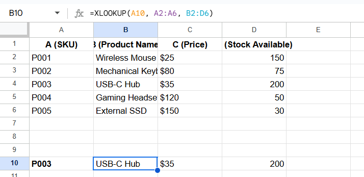
7. Google Sheet XLOOKUP(): Horizontal Lookup
The horizontal XLOOKUP() function works horizontally, which means we can use it to search for a value across a row rather than a column and return a similar value from another row.
Example:
You manage a sales team, and you have a table that records each salesperson’s total sales for different months. You want to quickly look up the total sales for a specific month using XLOOKUP in a horizontal format.
=XLOOKUP(A10, B1:M1, XLOOKUP(A11, A2:A4, B2:M4))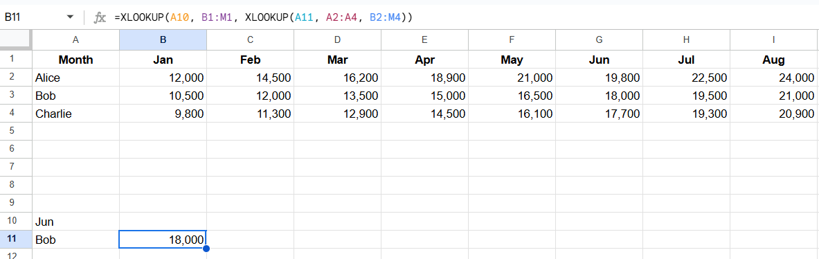
8. Using an ARRAY FORMULA
When working with smaller data sheets in Google Sheets, the XLOOKUP() function works fine, but when looking up values in larger data sets, we need to manually drag formulas down. ARRAYFORMULA in Google Sheets helps us apply functions like XLOOKUP, SUM, IF, etc. to entire columns or ranges automatically, so we don’t have to drag formulas down manually. We can use it for large datasets, ensuring our data updates dynamically as new entries are added.
Example:
Imagine you run an e-commerce store where you track products, their categories, and their discount percentages based on the category. Instead of manually applying formulas to each row, you can use ARRAYFORMULA with XLOOKUP to automate the process.
The formula for Discount%:
=ARRAYFORMULA(XLOOKUP(B2:B, E2:E4, F2:F4))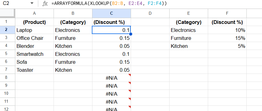
The formula for the Final Price:
=ARRAYFORMULA({"Final Price ($)"; 500 - (500 * C2:C / 100)})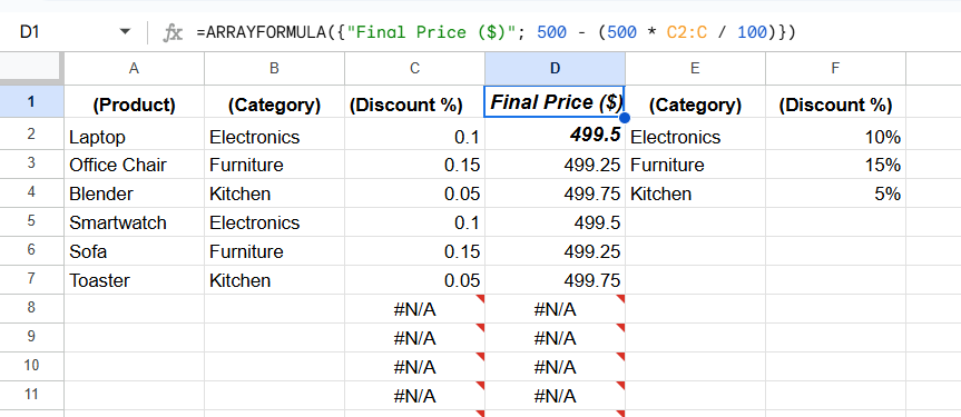
9. XLOOKUP() Search From Bottom to Top
The XLOOKUP function in Google Sheets allows searching from the last entry to the first using the optional search mode parameter.
- 1: It searches from the first to the last entry (default).
- -1: It searches from the last entry to the first.
- 2: It uses binary search (ascending order).
- -2: It uses binary search (descending order).
By default, XLOOKUP searches from top to bottom (like VLOOKUP), but sometimes, we may need to find the latest or least successful entry by searching in reverse.
Example:
Let’s assume that you have a sales report for multiple employees across different offices. You need to find the least successful employee’s sales in a particular office by searching from bottom to top instead of top to bottom.
Apply this formula as in the table:
=XLOOKUP(E2, B2:B9, C2:C9, , , -1)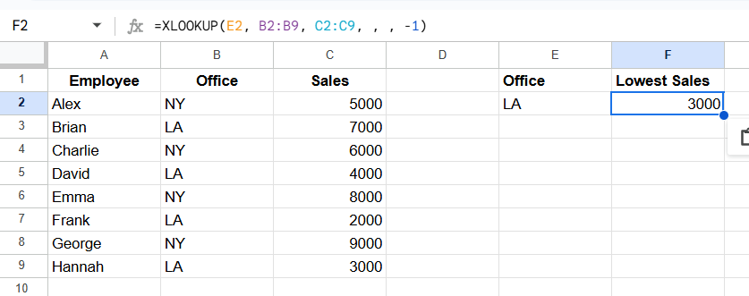
If you enter “LA” in E2, the formula will return 2000 (Hannah’s sales) since it searches from bottom to top and finds Hannah as the last occurrence of “LA”.
If you enter “NY” in E2, the formula will return 9000 (George’s sales).
10. Using Binary Search
Binary search is a powerful Google Sheets feature that speeds up searching in huge data sets. When we are searching through huge data sheets, it takes too long to look for values in each row separately. It divides the dataset in half at each stage, making it much easier for us to search through thousands of records.
Example:
Let’s assume that you have a sorted list of products based on their stock quantity. You want to quickly find the product details for a specific stock level using XLOOKUP with a binary search.
Formula:
=XLOOKUP(E2, C2:C8, A2:B8, "Stock level not found", ,-2)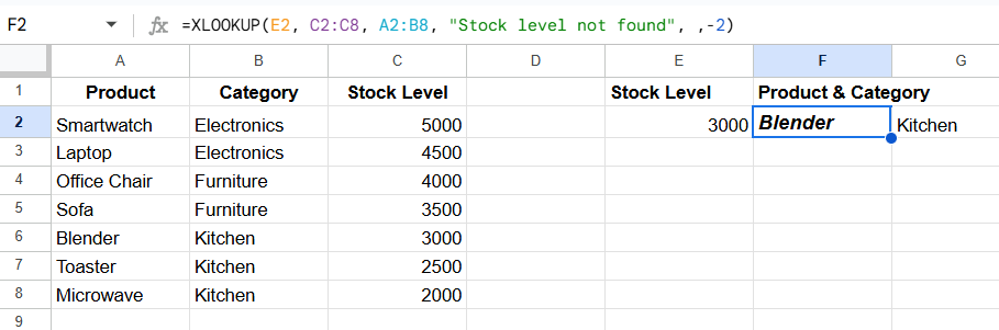
This list in the image is sorted in descending order by stock level (largest to smallest), which is crucial for binary search to work correctly.
Formula’s Breakdown:
- E2: The stock level you are searching for.
- C2:C8: The Stock Level column (lookup range).
- A2:B8: The columns containing Product & Category (return range).
- “Stock level not found”: The error message if no exact match is found.
- -2: Uses binary search, assuming the list is sorted in descending order.
If you enter 1000, it will return “Stock level not found”, since no product has 1000 stock available.
Wrap Up
By now, you’ve seen how versatile and powerful the XLOOKUP function is when managing data in Google Sheets. From simple lookups to advanced matching techniques, XLOOKUP simplifies your workflow and eliminates many of the limitations found in older Google Sheets lookup functions like VLOOKUP and HLOOKUP.
If you ever find XLOOKUP not working in Google Sheets, it’s often due to incorrect syntax, unsorted data for binary searches, or using unsupported wildcards. Always double-check your formula and data structure to fix common issues.
Compared to older methods, the debate between VLOOKUP vs XLOOKUP in Google Sheets leans in favor of XLOOKUP, thanks to its ability to search in any direction, return multiple results, and handle errors gracefully.
Now that you’ve had a chance to learn XLOOKUP step by step, you can confidently integrate it into your spreadsheets and take your data management skills to the next level.