How to Use VLOOKUP and IF Statement in Excel (Step-by-Step Guide with Examples)

If you worked with Excel, you may be aware of how difficult it is to manage huge data sheets on Excel. It’s difficult to handle and organize large datasheets in Excel, but don’t worry, we have a solution for you. We can use the VLOOKUP() function within an IF() statement to perform dynamic lookups depending on certain conditions. Using this method, you can simply manage big datasheets without problems. Here’s a breakdown of how to use VLOOKUP and IF statements together in Excel to solve a lot of problems.

VLOOKUP Function in Excel

We use the VLOOKUP (Vertical Lookup) function in Excel to look for a certain value in the first column of a range in a huge datasheet and return a value from another column in the same row.

Simply, you can use this function in Excel to look up a value and find items in a table or range by row. For example, you can use an employee ID to find an employee’s name.

Syntax:

=VLOOKUP(lookup_value,table_array,column_index_num,[range_lookup])

lookup_value: 

This is the value or data you’re looking for; it might be a number, a name, text, or a reference to a cell containing the search value.

table_array: 

This is a set of cells that you can use to locate the data or value you’re looking for. 

column_index_num: 

column_index_num specifies the column number in which you are conducting your research and looking for data. You can select any column to perform your search, such as Column 1, Column 2, or Column 3.

range_lookup: 

This parameter returns TRUE or FALSE depending on whether you require an exact or approximate match when returning your look-up data. If you do not specify the range_lookup, Excel will always return an approximate match or the FALSE value. When searching for a value in Excel, you can enter TRUE (or 1) for numbers and FALSE (or 0) for text. 

Example:

Let’s say you have a list of employees, their departments and names. Your goal is to quickly find which Employee’s ID 103 belongs to. Here’s your employees list with their departments and names. And now you want to know the department of a specific person using his/her ID. 

1. To start finding the ID, enter a lookup_value (in your case, ID 103) to find the department in any cell. 
2. Now select a cell and type =VLOOKUP().
3. Next, select the cell where the look_up value was entered.
4. Then, select the table_array of the table. 
5. Counting from the left, enter the number of a column from where you want to retrieve the data. 
6. Now, to get the exact match enter FALSE.
7. After all, hit the enter button
8. Now you can see in your data sheet that VLOOKUP() successfully retrieves the department of the person as below.

IF Function in Excel

We use the IF function in Excel to compare numbers and check them against the specified criteria. It allows you to make logical comparisons between a value and what you expect. Essentially, it checks whether a condition is met and returns one value if TRUE and another if FALSE.

Syntax:

=IF(logical_test, value_if_true, value_if_false)

• logical_test: The condition you want to evaluate (e.g., A1 > 50).
• value_if_true: The result if the condition is TRUE.
• value_if_false: The result if the condition is FALSE.

Example:

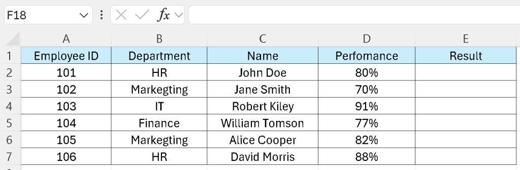
Let’s add perfomance column in the above list, and you want to determine if each person’s perfomance score passed or failed (passing score is 75%).

Select a cell E and type =IF(). You can print Pass if the perfomance score is above 75% and Fail if the score is below that.

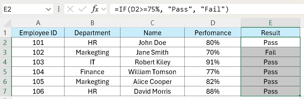
If the value in D2 is greater than 75%, Excel will return “Pass”, otherwise, it will return “Fail”.

=IF(D2>=75%, "Pass", "Fail")

Now you can hit the ENTER button to get the result and then drag or double click for the rest of results.

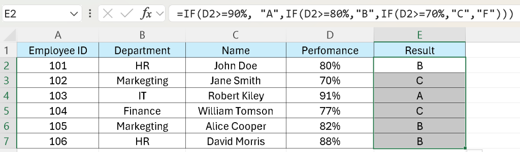
If you want describe a nested IF example to assign letter grades based on the scores.

You want to assign grades based on the following logic:

• 90% and above = A
• 80% to 89% = B
• 70% to 79% = C
• Below 70% = F

=IF(D2>=90%, "A",IF(D2>=80%,"B",IF(D2>=70%,"C","F")))

The results shows and explaines as below.

• If score ≥ 90% → A
• Else if score ≥ 80% → B
• Else if score ≥ 70% → C
• Else → F

How To Combine VLOOKUP and IF Statement in Excel?

Let’s look over how we can use VLOOKUP() and the IF() statement to solve many problems, streamline processes, and make things easier.

1. For Conditional Lookups Or to Match a Specific Value

You can use VLOOKUP() and IF() statements for conditional formatting and to match a specific value in the table. To return different results based on criteria, you have to first start with an IF() statement and then use VLOOKUP inside it.

First, write IF() statement =IF() and then write VLOOKUP inside it.

Example:

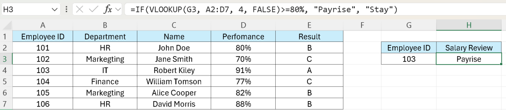
From the employee table with perfomance score, you want to review an employee’s salary basend on a threshold.

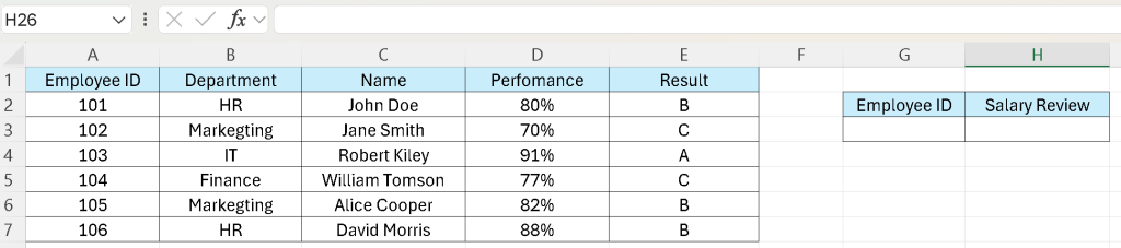
First, you have to create columns for Employee ID you look for and salary review column.

=IF(VLOOKUP(G3, A2:D7, 4, FALSE)>=80%, "Payrise", "Stay")

• Enter the VLOOKUP() function looks for ID from G3 column which contains the Employee ID you want to look for.
• Search range is A2 to D7, all range of data that is relevant to the salary review.
• The perfomance score is 4th column, so the number should be 4, enter FALSE to look for exact match.

• Now, add the IF() statement returns “Payrise” If the score is >=80%, otherwise “Stay”.

If you want to check which employee should get payrise, and you want the output in Yes or No (Yes for payrise and No for stay as the current salary) then you can write this formula as below:

=IF(VLOOKUP(G3, A2:D7, 4, FALSE)>=80%, "Yes", "No")

2. For Error Handling

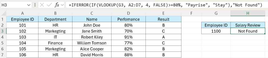
You can also combine the VLOOKUP() with the IF() statement for error handling. To use them together, you must first use the IFERROR() statement, along with the IF() and VLOOKUP() statements inside it. 

Let us use the previous example to see how this can be done practically.

• Assume you have a large table of employees with the performance score and want to display a custom message instead of an error when an employee ID is not found. 
• First select a cell and enter the IF() + VLOOKUP() formula to determine if an employee is required payrise or not.
• Add the IFERROR() outside of the formula, now you can use this to handle the error.

=IFERROR(IF(VLOOKUP(G3, A2:D7, 4, FALSE)>=80%, "Payrise", "Stay"),"Not Found")

Now you can see that it returns employee not found rather than showing an error.

– Return 0 If Not Found

Use this formula if you want to return 0 instead of showing “Employee ID Not Found” and an error.

=IFERROR(IF(VLOOKUP(G3, A2:D7, 4, FALSE)>=80%, "Payrise", "Stay"),"0")

– Return Blank Cell If Not Found 

=IFERROR(IF(VLOOKUP(G3, A2:D7, 4, FALSE)>=80%, "Payrise", "Stay")," ")

3. Dynamic Column Indexing

One limitation of VLOOKUP is that the column index number must be manually defined. If your data structure changes, the column number may become incorrect. 

You can also combine IF() and VLOOKUP() to dynamically select the column index. To choose different columns based on a condition, you have to first use an IF() statement and then use VLOOKUP() within it.

Example:

You have a product table where column you want to look up a product’s price or product name based on whether the price is above or below a certain threshold, such as $100.

Select a cell and enter the following formula:

=IF(VLOOKUP(A9, $A$9:$C$14, 3, FALSE) > 100, VLOOKUP(A9,$A$9:$C$14, 2, FALSE), VLOOKUP(A9,$A$9:$C$14, 3, FALSE))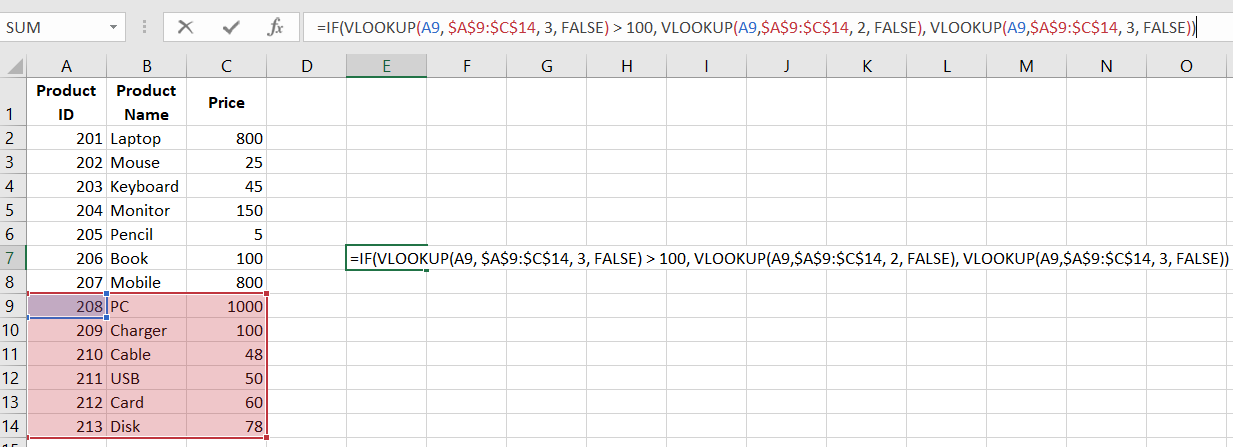

Breaking Down Formula’s Working:

• VLOOKUP(A9, $A$9:$C$14, 3, FALSE): It looks up the product ID in A9 and returns the price from column C.
• The IF() statement checks if the price was greater than $100.
•  VLOOKUP(A9, $A$9:$C$14, 2, FALSE): If true, the formula returns the product name:
• VLOOKUP(A9, $A$9:$C$14, 3, FALSE): If false, the formula returns the product price: 

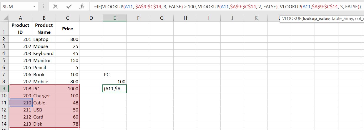
As you can see, you can extract the needed information depending on certain conditions by simply combining two formulas, IF() and VLOOKUP().

Note: One of the most important things you must do every time you execute a task is to update the column index number in the formula in which you are performing your research. As you can see at the top, the formula has changed for the new research.

Advanced Level IF() and VLOOKUP Techniques You Need to Know!

After mastering the basics, you can progress to more advanced techniques to make large projects more manageable and flexible.

1. Combining Multiple Criteria with VLOOKUP() and IF()

We can also use VLOOKUP() with IF() to combine various criteria. When looking up data using multiple criteria, you can use these two statements to ensure that all conditions are met.

Example:

Let’s assume you have a table with employee data, including their total years of experience and performance rating. You want to check if an employee is eligible for a promotion, which requires at least 5 years of experience and a performance rating of ‘Excellent’.

Here’s your employee data:

Now, in a new column named “Promotion Eligibility”, enter the following formula:

=IF(AND(VLOOKUP(A2, $A$2:$C$6, 2, FALSE) >= 5, VLOOKUP(A2, $A$2:$C$6, 3, FALSE) = "Excellent"), "Eligible", "Not Eligible")

Breaking Down Formula’s Working:

1. VLOOKUP(A2, $A$2:$C$6, 2, FALSE) >= 5: This checks if the employee has at least 5 years of experience.
2. VLOOKUP(A2, $A$2:$C$6, 3, FALSE) = “Excellent”: This checks if the performance rating of employee 201 was ‘Excellent’.
3. AND(): It ensures both conditions were met.
4. IF(): It returns “Eligible” if both conditions were true, otherwise returns “Not Eligible”.

2. Using Both for Calculation

You can also combine VLOOKUP() and IF() to perform calculations: first, use VLOOKUP() to find a value, and then use IF() to conduct calculations on that value.

Example:

Assume that you have a table with customer orders and their total bill amounts and you want to apply a 15% discount to orders above $500.

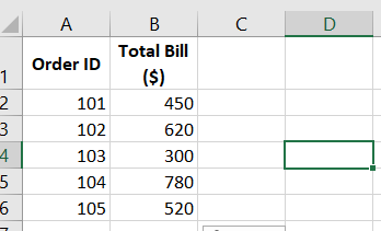
Now you have to create another column named Discount” and enter the following formula to display the discount.

=IF(VLOOKUP(A2, $A$2:$B$6, 2, FALSE) > 500, VLOOKUP(A2, $A$2:$B$6, 2, FALSE) * 0.85, VLOOKUP(A2, $A$2:$B$6, 2, FALSE))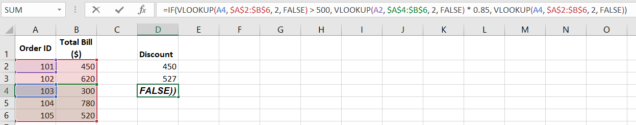

Now you can see that you can find the discount for all other  IDs by using the same formula and simply dragging it down to apply to all orders.

Breaking Down Formula’s Working:

• VLOOKUP(A2, $A$2:$B$6, 2, FALSE): It retrieves the total bill for the ID 101.
• IF(VLOOKUP(A2, $A$2:$B$6, 2, FALSE) > 500, …, …): It checks if the total bill was greater than $500.
• VLOOKUP(A2, $A$2:$B$6, 2, FALSE) * 0.85: As the condition was true, it applies a 15% discount by multiplying the bill amount by 0.85.
• VLOOKUP(A2, $A$2:$B$6, 2, FALSE): Printed the actual bill where the condition was not true.

3. Matching Lookup Values with the Highest Price

We can also use these two functions to find the highest value in a larger data sheet and determine whether there is a highest matching value in the data we have input. 

Example:

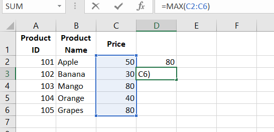
Let’s assume that you have a price list of different products in an Excel sheet and you want to check if a specific product has the highest price in the list.

In this method, you will use the MAX function to find the highest price in the given data. Then, you will compare this highest price with the price of a specific item using the IF and VLOOKUP functions.

• First of all click on an empty cell where you want to display the highest price.
• Now enter this formula to find out the highest price:

=MAX(C2:C6)

• Now press enter and this will return the highest price in the data set. As you can see in the image it has returned the highest value which is 80.

Now let’s say you want to check if the price of a Banana is the highest.

• Click on another empty cell and type this formula, this will return the Banana’s price

=VLOOKUP(102, A2:C6, 3, FALSE)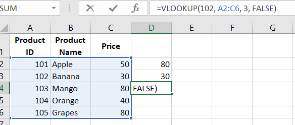

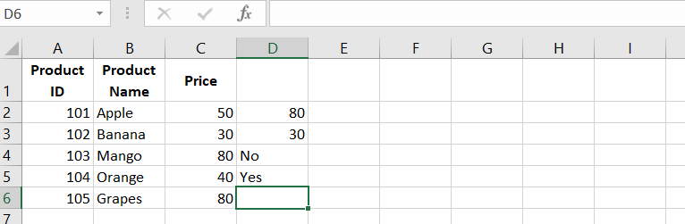
• Now, select another empty cell and enter this formula and press enter.

=IF(VLOOKUP(103, A2:C6, 3, FALSE) >= MAX(C2:C6), "Yes", "No")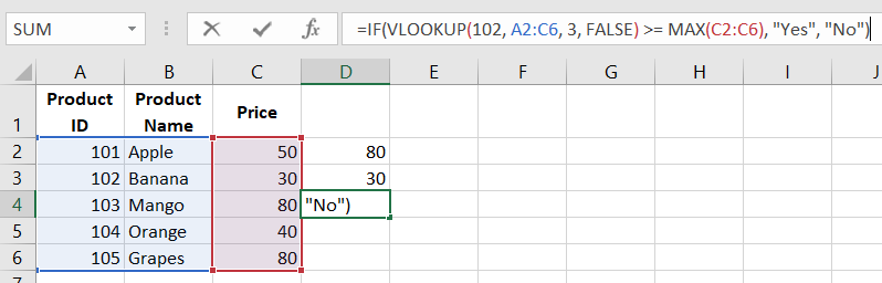

As you can see it returns “NO” because the price of banana was not equal to the highest price. But if you select Mango instead of Banana then it will return “Yes” because the price of Mango is Equal to the highest price. 

Formula’s Breakdown:

• VLOOKUP(102, A2:C6, 3, FALSE): It finds the price of Banana (ID: 102).
• MAX(C2:C6): It finds the highest price in the dataset (80).
• IF(VLOOKUP >= MAX, “Yes”, “No”): It compares the product’s price with the highest price and returns:
  • “Yes” if it is the highest.
  • “No” if it is not.

Conclusion

So, now you know how to use VLOOKUP and IF statements together in Excel to simplify your data management. Whether you want to look up values, apply conditional logic, handle errors, or perform advanced calculations, you can easily do it with these functions. Instead of manually searching through large spreadsheets, you can automate tasks and get accurate results in seconds. Try applying these formulas to your own datasets, and you’ll see how much time and effort you can save. If you ever get stuck, just revisit these examples, and you’ll be back on track in no time!