5 Easy Ways to Combine Two Excel Columns (With Examples)

I’ve been working with Excel for years, and one of the most common questions I get is: “How do I combine two columns in Excel?” Maybe you’ve got first names in column A and last names in column B. Or maybe you’re trying to combine city and state data for a mailing list.

Whatever the reason, I’ve got you covered. Here are 5 methods I use all the time—from super simple to more advanced.

Quick Answer

Just need a fast solution? Type =A2&" "&B2 in an empty cell. That’s it. The & symbol joins your cells together, and " " adds a space between them. Press Enter, drag down, and you’re done.

Want something fancier? Keep reading—I’ll show you when to use Flash Fill, TEXTJOIN, and even Power Query.

Why would you even want to combine columns?

There are many practical reasons why you might want to merge two columns in Excel:

• Merging first and last names – Creating a full name column from separate first and last names.
• Combining addresses – Merging street, city, and state into a single column.
• Unifying data for reports – Merging different columns for a clean data structure.
• Creating unique IDs – Combining order numbers and customer IDs for better tracking.
• Cleaning up messy data– Making unstructured data more readable and useful.

5 ways to combine columns (from easiest to most powerful)

Method	Best For	Difficulty
Ampersand (&)	Quick and simple text merging	Beginner
CONCAT	Merging text with flexibility	Beginner
TEXTJOIN	Combining multiple columns with delimiters	Intermediate
Flash Fill	One-time merge without formulas	Beginner
Power Query	Automating merging for large datasets	Advanced

Let’s dive into each method with step-by-step instructions.

Method 1: Using the Ampersand (&) Formula (Fastest Way)

This is how I do it 90% of the time. It’s fast, it works everywhere, and you don’t need to remember complicated function names.

Example: First Name + Last Name

First Name	Last Name	Full Name
John	Doe	John Doe
Jane	Smith	Jane Smith
Mark	Johnson	Mark Johnson

Let’s say A2 has “John” and B2 has “Doe” as above. Here’s the formula:

=A2 & " " & B2

What’s happening here:

• A2 grabs the first name
• " " adds a space (don’t forget this or you’ll get “SarahJohnson”)
• B2 grabs the last name

How to do it

1. Click any empty cell (like C2)
2. Type the formula exactly as shown above
3. Hit Enter
4. Grab the little square at the bottom-right of the cell and drag down

Example with comma:

1. Suppose you have data as below.
2. To merge the values from cells A2, B2, and C2 with commas separating them, you can use the following formula:

=A2 &", "& B2 &", "& C2

First, select D2  and enter the formula above.

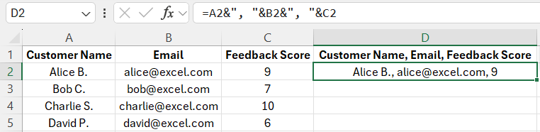
Now you can see in the image above that the data of two cells is merged and separated by commas in one cell without losing any value or data. 

3. To fill the remaining cells, select D2, then either copy and paste (Paste Special > Values), or use the fill handle—the small dot in the bottom-right corner—and drag it down.

The good and the bad

• Good: Super fast, works in every version of Excel, easy to remember
• Bad: If you’re combining 5+ things, the formula starts looking messy

Method 2: CONCAT (same thing, fancier name)

Honestly? This does the exact same thing as the ampersand method. But some people prefer it because it looks more “official.”

The formula

=CONCAT(A2, " ", B2)

Older Excel (before 2016)

=CONCATENATE(A2, " ", B2)

Click on an empty cell where you want the combined data.

• Type the above formula: using CONCATENATE function for Excel 2016 and older / CONCAT function for Excel 2019 and later versions
• Press Enter and drag the fill handle down to apply it to other rows.

When I use this

When I’m working on a shared file and want the formulas to look professional. Or when I’m combining lots of things and & starts looking cluttered.

The good and the bad

• Good: Easier to read in complex formulas
• Bad: Not really faster than &, and you have to remember the function name

Method 3: TEXTJOIN (the secret weapon for multiple columns)

This is where things get interesting. TEXTJOIN is perfect when you’re combining 3 or more columns, and especially when some of those columns might be blank.

Example: First, middle, and last name

Let’s say you have:

• A2: “Jane”
• B2: “” (middle name is blank)
• C2: “Smith”

Here’s the magic formula:

=TEXTJOIN(" ", TRUE, A2, B2, C2)

What this does:

• " " = separator (I’m using a space)
• TRUE = ignore blank cells (so you won’t get “Emily Rodriguez” with two spaces)
• A2, B2, C2 = the cells you’re combining

First Name	Middle Name	Last Name	Full Name
John	A.	Doe	John A. Doe
Jane		Smith	Jane Smith
Mark	B.	Johnson	Mark B. Johnson

The good and the bad

Good: Handles blanks like a champ, great for 3+ columns

Bad: Only works in Excel 2016 or newer

Method 4: Flash Fill (no formulas required!)

Okay, this one blows people’s minds. Flash Fill is Excel’s way of saying, “I see what you’re doing, let me finish it for you.”

How it works

1. Let’s say column A has first names and column B has last names
2. In column C, type out the first result manually (like “John Doe”)
3. Press Enter and click the next cell
4. Hit Ctrl + E (or go to Data → Flash Fill)
5. Watch Excel magically fill in the rest

When I use Flash Fill

• Quick one-time cleanup jobs
• Preparing data for a report or export
• When I just want the results and don’t care about formulas

Important warning

Flash Fill creates static results. If you change “John” to “Jonathan” in column A, your Flash Fill result won’t update. For that, you need a formula.

The good and the bad

Good: Stupidly fast, no formula knowledge needed

Bad: Results don’t update if your data changes

Method 5: Power Query (for the pros)

If you’re dealing with large files or need to merge columns repeatedly, Power Query is worth learning. It’s like setting up a reusable recipe.

The steps

1. Click anywhere in your data
2. Go to Data → From Table/Range
3. Hold Ctrl and click the two columns you want to merge
4. Go to Transform → Merge Columns
5. Pick your separator (space, comma, dash, whatever)
6. Click Close & Load

Now whenever you refresh your data, the merge happens automatically.

The good and the bad

• Good: Repeatable, handles huge datasets, looks impressive in meetings
• Bad: Takes a bit of practice to learn

Handling tricky situations

Need a dash instead of a space?

If your columns contain numbers, Excel treats them as text when using &.

=A2 & "-" & B2

Result: “Order-12345”

Want to smash things together with no separator?

If you don’t need a separator, simply remove " " from the formula.

=A2 & B2

Result: “JohnDoe” or “CA94102”

Got messy data with extra spaces?

Wrap your formula with TRIM to clean it up:

=TRIM(A2 & " " & B2)

Mistakes I see all the time (and how to avoid them)

Forgetting the space

If you type =A2&B2 without the " ", you get “JohnSmith” instead of “John Smith”. Always add your separator!

Double spaces when cells are blank

If B2 is blank and you use =A2&" "&B2, you might get “John ” with a trailing space. Fix it with TEXTJOIN or TRIM.

Thinking Flash Fill updates automatically

It doesn’t. Flash Fill is a one-time thing. If your source data changes, you need to re-run it or switch to a formula.

My recommendations (where to start)

If you’re new to this:

• Start with & for simple stuff
• Try Flash Fill when you just need quick results
• Learn TEXTJOIN when you’re ready to level up

If you work with Excel regularly:

• Master TEXTJOIN for handling blanks
• Learn Power Query for repeatable workflows

That’s it! Pick the method that fits your situation and you’ll be combining columns like a pro in no time.

Got questions? Drop them below. I’m always happy to help troubleshoot Excel weirdness.

If you want to explore more about Formulas in Excel, check out this comprehensive guide for in-depth explanations and practical examples.