Navigating large spreadsheets in Microsoft Excel can be challenging, especially when headers or key identifiers disappear as you scroll. The Freeze Panes feature solves this problem by locking specific rows or columns in place, ensuring essential data remains visible no matter where you scroll.
In this guide, we’ll walk you through how to freeze panes in Excel step by step, including freezing rows, columns, and multiple panes simultaneously.
What is Freezing Panes in Excel?
Freezing panes allows you to lock specific rows or columns in place while scrolling through your data. This feature is particularly useful for:
- Tracking Headers: Keep column titles visible.
- Monitoring Key Identifiers: Lock reference columns or rows.
- Simplifying Navigation: Easily compare data across large datasets.
By using Freeze Panes, you’ll improve productivity and reduce errors during data analysis.
Preparing Your Worksheet for Freezing Panes
Before freezing panes, ensure your worksheet is ready:
- Open Your Excel File: Load the spreadsheet you want to work on.
- Identify Key Rows or Columns: Determine which headers or reference points you need to keep visible.
Proper preparation prevents unnecessary adjustments later.
How to Freeze Rows and Columns in Excel
How to Freeze the Top Row in Excel?
Freezing the Top Row is ideal for locking column headers in place.
Steps to Freeze the Top Row:
- Open your Excel workbook.
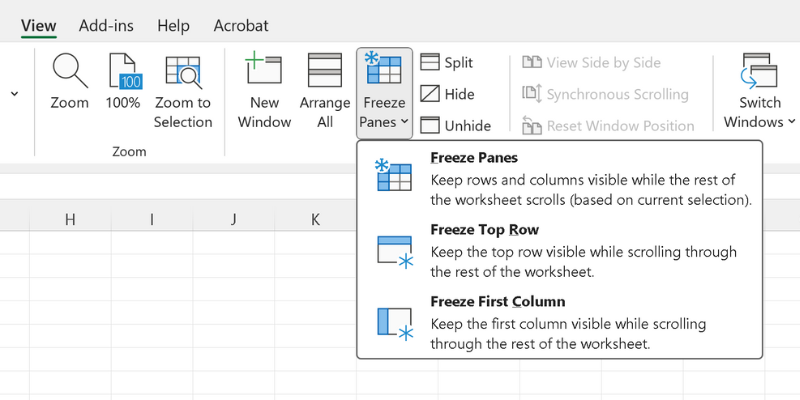
- Click on the View Tab located at the top.
- Find the Freeze Panes dropdown menu.
- Select Freeze Top Row from the list.
Now, as you scroll down, the top row will remain fixed in place.
Use Case: Tracking column headers in financial reports or data tables.
How to Freeze the First Column?
Freezing the First Column keeps key identifiers (e.g., names, IDs) locked while scrolling horizontally.
Steps to Freeze the First Column:
- Go to the View Tab.
- Open the Freeze Panes dropdown menu.
- Select Freeze First Column.
The first column will now remain visible as you scroll across the sheet.
Use Case: Keeping reference IDs or customer names visible during data navigation.
How to Freeze Rows and Columns Simultaneously?
For complex datasets, you might need to freeze both rows and columns at the same time.
Steps to Freeze Rows and Columns:
- Click on the cell below the row and to the right of the column you want to freeze.
- Example: To freeze the first row and column, click on cell B2.
- Go to the View Tab > Freeze Panes.
- Select Freeze Panes from the dropdown list.
This will lock the rows above and columns to the left of the selected cell.
Use Case: Analyzing large datasets with both row headers and key identifiers.
Video by Microsoft Excel on YouTube
How to Unfreeze Panes in Excel?
When you’re done with frozen panes, you can easily unfreeze them.
Steps to Unfreeze Panes:
- Navigate to the View Tab.
- Click on the Freeze Panes dropdown.
- Select Unfreeze Panes.
All locked rows and columns will be released, and scrolling will return to normal.
Practical Applications of Freezing Panes
Data Analysis:
Keep header rows visible for context during analysis.
Financial Reports:
Ensure row or column labels stay in view while scrolling through financial data.
Project Management:
Lock key identifiers in project timelines or tracking sheets.
Inventory Management:
Freeze item names or product IDs while reviewing stock levels.
Freezing panes enhances clarity and reduces errors across various data-intensive tasks.
Benefits of Using Freeze Panes
Improved Navigation:
Easily track data across large sheets.
Reduced Errors:
Avoid misreading or overlooking critical information.
Enhanced Productivity:
Spend less time scrolling and searching.
Better Data Comparison:
Effortlessly compare rows and columns.
Tips for Using Freeze Panes Effectively
- Always identify key rows and columns before freezing.
- Use Unfreeze Panes if navigation feels restricted.
- Combine Freeze Panes with Split View for advanced data tracking.
Conclusion
Freezing panes in Excel is an essential feature for anyone working with large datasets. Whether you need to freeze the top row, first column, or a combination of both, mastering this feature ensures better clarity, smoother navigation, and increased productivity.
Start using Freeze Panes today to simplify your data management tasks and prevent costly mistakes.