
XLOOKUP() is an advanced search function in Microsoft Excel that allows you to search for values such as VLOOKUP, HLOOKUP, and INDEX-MATCH. However, XLOOKUP is more efficient than other functions with limitations, such as VLOOKUP().
Excel introduced the XLOOKUP() function in its 365 and 2019 versions. XLOOKUP makes it easier to search for values in a dataset and provides more flexibility than previous versions.
Here’s a quick overview of the Excel XLOOKUP function, its syntax, and the top seven ways it can improve Excel workflow efficiency.
Excel XLOOKUP( ) Purpose
The main reason we use XLOOKUP is to search for data from a larger data source. It compares and returns the values from the larger data sets. XLOOKUP() finds the exact or appropriate match in the datasheet, and if there are several matching values, it returns the last or first matching value, based on the formula inputs.
XLOOKUP() can find values vertically and horizontally using several criteria, and it can even return an entire column or row of data rather than just one value. Finally, Microsoft Excel has created a powerful function that can handle all of the frustrating problems and limitations of other LOOKUP() functions, such as VLOOKUP().
Syntax
= XLOOKUP(lookup_value, lookup_array, return_array, [if_not_found], [match_mode], [search_mode])- lookup_value: This is the value that we will be looking for in our data sheet.
- lookup_array: The range or array means rows and columns, e.g; A2:D8 in which we are searching for the lookup_value.
- return_array: This will be the range or array from which our desired matching value will be returned.
- [if_not_found] (Optional): The value returned if no match is found.
- [match_mode] (Optional): Specifies the type of match (Exact, Approximate, or Wildcard match).
- 0 or omitted (default): Exact match. If not found, an #N/A error will be returned.
- -1: Exact match or next smaller. If an exact match is not found, it will return the next smaller value.
- 1: Exact match or next larger. If an exact match is not found, it will return the next larger value.
- 2: Wildcard character match.
- [search_mode] (Optional): This mode defines the search order (Top-to-Bottom, Bottom-to-Top, Binary Search).
- 1 or omitted (default): This mode will search for a value from the first column or row to the last column or row.
- -1: This mode will search for a value in reverse order, from the last column and row to the very first.
- 2: This mode will perform a binary search on the data in ascending order.
- -2: This mode will perform a binary search on the data in descending order.
XLOOKUP Excel: why use it?
XLOOKUP was launched to give you more power over your calculations. Here’s why it’s a smart addition to your spreadsheets:
- It merges the functionality of both VLOOKUP and HLOOKUP, enabling you to retrieve data across rows and columns alike.
- You get control over a lot of things while using XLOOKUP, like error message, match settings, and even the order in which the array will be scanned.
- With XLOOKUP, there’s no restriction on where your lookup and return ranges are positioned, they can be placed independently. Even better, it can effortlessly return values from several columns at once.
- Plus, it’s built-in support for arrays makes it ideal for handling complex and dynamic calculations.
1. Excel XLOOKUP: Basic Exact Match
Suppose you are a teacher and have a table that lists students’ marks and their corresponding grades. You want to quickly find a student’s grade based on their marks.
This table is in Excel Columns A and B, where:
- Column A contains Marks
- Column B contains Grades
Step 2: Use XLOOKUP to Find Grade
Let’s say a student scored 75 marks, and you need to find their grade.
Formula:
=XLOOKUP(75, A2:A8, B2:B8, "Grade Not Found", 1)Formula’s Breakdown:
- 75: The marks we are looking up
- A2:A8: The lookup range (Column A, where marks are stored)
- B2:B8: The return range (Column B where grades are stored)
- “Grade Not Found”: Custom message if marks are not found
- 1 (Approximate Match): Finds the nearest smaller value if an exact match is not available
2. Looking Horizontally and Vertically
Before Excel introduced XLOOKUP, we used the VLOOKUP function to look up a value vertically and the HLOOKUP to look up a value horizontally. However, the usage of the XLOOKUP function makes this process much easier. We can now search for a variable vertically and horizontally using only the XLOOKUP method. It means you can look at a value in both rows and columns and then return the value from another row and column.
Let us take an example of this.
Example: Vertical LOOKUP
Let’s assume that you’re managing multiple projects, and you want to quickly find the deadline for a specific project using XLOOKUP.
Use this formula:
=XLOOKUP(D2, A2:A6, B2:B6, "Project Not Found")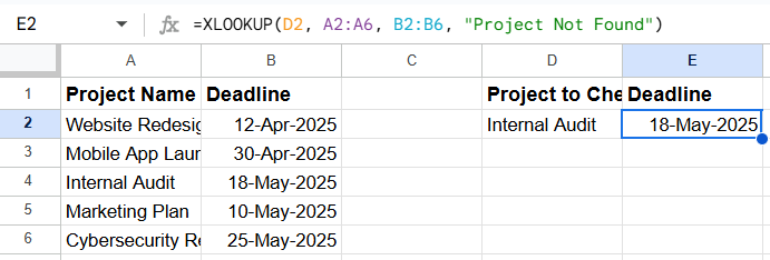
As you can see from the image, the formula has returned the matching value for the input. If the corresponding value is not found in the table, it will return “Project Not Found” rather than an error.
Horizontal LOOKUP:
You work in Finance at a marketing agency. Each department (Marketing, HR, Operations) submits its quarterly budgets. This data is organized horizontally across quarters.
Now, your boss asks about the budget used in department Q3.
You want a dynamic way to pull that number, where you can change the department and quarter, and Excel gives you the right figure instantly.
You can use this formula
=XLOOKUP(B7, B1:E1, XLOOKUP(B6, A2:A4, B2:E4))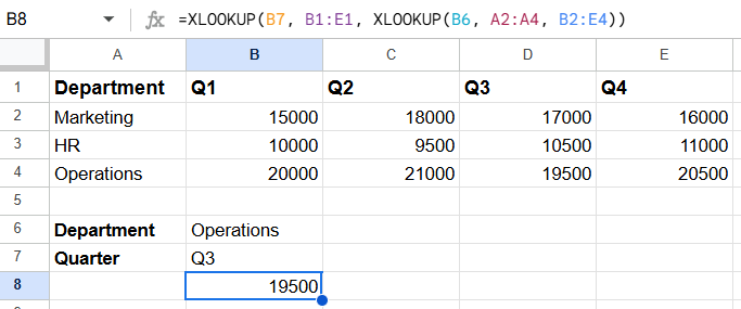
Formula’s Breakdown:
- XLOOKUP(B6, A2:A4, B2:E4): This finds the entire row of the department selected in B6 (e.g., “Operations”).
- XLOOKUP(B7, B1:E1, …): This looks across the header row to find the matching quarter (e.g., “Q3”) and returns the corresponding value from the row found above.
3. Missing Value or Product Not Found ( # N/A Error Handling)
When the Excel XLOOKUP function can’t find a matching value in the data, it returns a #N/A error, which can be inconvenient for you as a newbie. However, you can correct these problems by quite changing the formula. Instead of playing the error, this will display a user-friendly message. Consider the vertical LOOKUP example, where we have added “Project Not Found” at the end of the formula.
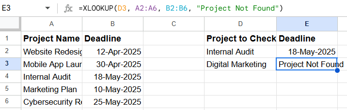
As you can see in the picture, we are looking for a value that does not exist in the data. Instead of displaying a #N/A error, it returned “Project Not Found” in the output area.
4. Left XLOOKUP
As you know, VLOOKUP and HLOOKUP do not allow us to look above and left. You can only look for values to the right of the data sets. However, XLOOKUP has transformed the game. Now, with XLOOKUP, you can easily look at a value to the left of the data sheet.
Let us use an example to better understand this.
Example:
Assume that you’re working in a customer service department and that you have a list of customer feedback scores along with their corresponding names and email addresses.
Now, let’s say you only have the feedback score and want to retrieve the customer’s name associated with that score.
With traditional VLOOKUP, this would be an issue if the name column is to the left of the feedback score column. But with XLOOKUP, you can easily perform this reverse lookup without rearranging your data.
You can use this formula:
=XLOOKUP(E2, C2:C10, A2:A10, "Name Not Found")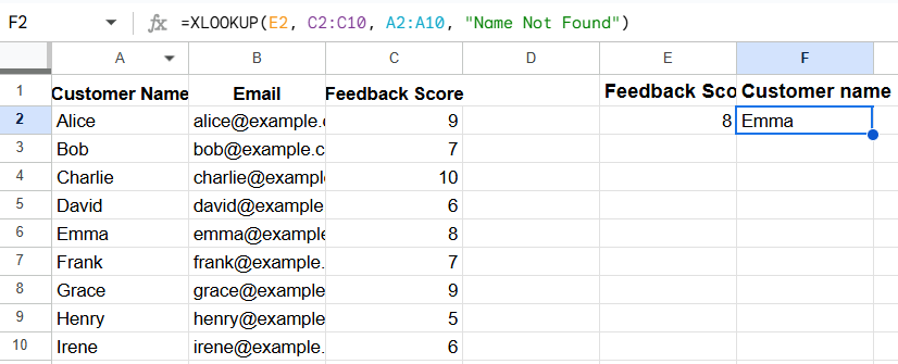
As you can see, it has returned the value from the left of the lookup value. If it can’t find the data on the sheet, it will return “Name Not Found” rather than a #N/A error.
5. Excel XLOOKUP Approximate Match
The fifth argument of the XLOOKUP function is the matching mode, which is set to 0. And when we look for a value, the matching mode will automatically look for an exact match. If this mode does not find the exact match value, it will return an error.
So, when we use the approximate match mode, it will continue to hunt for the exact match value. When it can’t find it, it will look for an approximate matching number that will be lower or higher than the exact match value, depending on the formula you entered.
Example:
Let’s assume that you’re working in a logistics company, and you have a shipping rate chart based on predefined weight brackets. Customers may send packages with weights that don’t exactly match your table. To determine the correct rate, you want to find the closest weight bracket that’s equal to or less than the actual package weight.
For Nearest Lowest Value:
=XLOOKUP(D2, A2:A6, B2:B6, "Not Found", -1)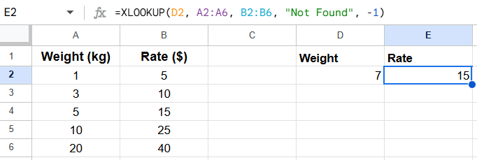
As you can see in the image, the formula has returned $15, because 7 falls between 5 and 10, and the closest smaller value is 5.
For Nearest Highest Value:
=XLOOKUP(D3, A2:A6, B2:B6, "Not Found", 1)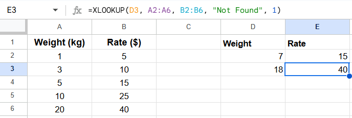
As you can see that the formula has returned $40, because the next higher weight bracket after 18 kg is 20 kg.
Formula’s Breakdown:
- D3: Cell where you input the actual package weight
- A2: A6: Weight bracket column
- B2:B6: Corresponding rate column
- “Not Found”: Custom message if no match is found
- -1: This tells XLOOKUP to find the nearest smaller value if an exact match isn’t found.
- 1: This tells XLOOKUP to find the nearest Highest value if an exact match isn’t found.
6. Excel XLOOKUP Wildcard Match
Wildcard match means you want to find a value based on half output, so to do that, just use 2 in the match mode, then the XLOOKUP function will look for wildcard characters according to this mode.
Wildcard matches indicate that the output can be found with the partial input using these characters.
Let’s look at an example to better comprehend the scenario.
Using * (Asterisk):
Imagine you’re managing an inventory system for a retail business. Each product has a unique product code followed by extra identifiers. You want to find the product category using only a partial code prefix since full codes are long and inconsistent.
You can use XLOOKUP with a wildcard (like *) to match any product code that starts with a known prefix.
Let’s say you only know the code starts with “ELX” and you want to find its category.
You can use this formula:
=XLOOKUP("ELX*", A2:A6, B2:B6, "Category Not Found", 2)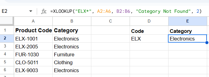
Using ? (Question Mark):
You want to match a product code that follows the pattern “FUR?X”, where the ? Represents exactly one unknown character between “FUR” and “X”.
In this case, it would match “FUR?X-5000”.
=XLOOKUP("FUR?X*", A2:A7, B2:B7, "Category Not Found", 2)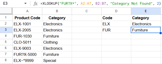
Using ~ (Tilde):
The ~ is used when you want to search for the actual wildcard characters like * or ? as literal characters, not as wildcards.
You want to look up a code that contains an asterisk like “ELX*9999” (not a wildcard).
=XLOOKUP("ELX~*9999", A2:A8, B2:B8, "Category Not Found", 2)
7. Excel XLOOKUP: Searching From Bottom to Top
If you want to search for a value from bottom to top, Excel XLOOKUP can help. The sixth mode of the XLOOKUP is search mode, which allows you to look for a value from the bottom up.
Let us take an example of this.
Example:
Assume that you’re managing a project tracking sheet where tasks are assigned to employees over time. Each time a task is assigned, it’s recorded in a new row. Now, you want to quickly find the most recent task assigned to a specific employee, searching from bottom to top.
This is where the search mode -1 in XLOOKUP becomes useful.
Use this formula:
=XLOOKUP(E2, B2:B10, C2:C10, "No Task Found", , -1)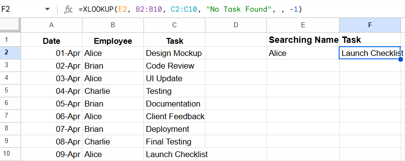
If you remove -1, Excel will return the first task assigned to Alice (“Design Mockup”)
8. Excel XLOOKUP: Return Multiple Results
VLOOKUP and other Lookup functions can only return one value as search results. But using the Excel XLOOKUP function, you can return multiple values at once.
Example:
Let’s assume that you work at a law firm that manages detailed records of all clients in a case tracking system. Now, whenever you enter a specific Client ID, you want to automatically retrieve all key details about the client using just one XLOOKUP formula.
=XLOOKUP(A9, A2:A6, B2:D6)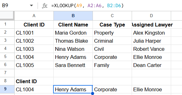
9. Excel XLOOKUP With Multiple Criteria
You can use XLOOKUP to return results based on various conditions and criteria, just as you can get multiple results based on a single output. It means that you can specify particular conditions in the formula, and it will produce results based on these.
Example:
Let’s take the previous example and assume that you want to retrieve all details about a client based on multiple criteria like Client ID, Case Type, and Assigned Lawyer.
You can use this formula:
=XLOOKUP(1, (A2:A6=A9)*(C2:C6=B9)*(D2:D6=C9), B2:D6, "Client Not Found")10. Nested XLOOKUP
A Double XLOOKUP (also called a nested XLOOKUP or 2-way lookup) is used when you want to find a value based on both a row and a column, like finding the value found where a certain row and a particular column intersect within a table.
Example:
You work in sales. You have a table that shows how much each salesperson sold in each quarter.
Now, you want to find out how much “Sarah” sold in “Q2”.
Use this formula:
=XLOOKUP(G1, A2:A5, XLOOKUP(G2, B1:E1, B2:E5))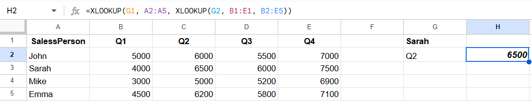
Formula’s Breakdown:
- The inner XLOOKUP looks for Q2 in B1:E1 and returns that entire column (e.g., the Q2 column).
- The outer XLOOKUP looks for salesperson Sarah in A2:A5 and returns the value in the Q2 column for Sarah (which is 6500).
Common Excel XLOOKUP Errors
Here are some common XLOOKUP errors that you could face while working.
Not Available:
If your formula is not working in Excel, it could be because XLOOKUP is not accessible in your version. You can only get XLOOKUP in Microsoft 365 and Excel 202, because it’s not available in other Excel versions. So, if you find a problem, you can check your Excel version and upgrade it.
Giving Wrong Results
Sometimes you might get incorrect results. This could be due to incorrect input and output ranges. To avoid this issue, you should always check both ranges.
Return #N/A Errors
When using XLOOKUP, the majority of users encounter #N/A errors. This happens when the value is not found in the data you are searching for. To resolve this issue, use the “Not Match Found” and “Approximate Match” conditions.
Returns #VALUE error
If you receive this error, it could be because you are attempting to match data from a row and return something from a column. Excel becomes confused because the contours of the data do not match. So you can look at the formula and adjust the input and output ranges.
Returns #REF Error
This is also a common problem in Excel, which you can face when working with XLOOKUP. The error occurs only when you try to search for a value from two separate workbooks, one of which is closed. To overcome this problem, you must open both workbooks.
XLOOKUP VS VLOOKUP
Here’s a quick comparison of XLOOKUP with VLOOKUP so that you can observe why you should replace VLOOKUP with XLOOKUP.
| Feature | XLOOKUP | VLOOKUP |
| Lookup Direction | Both directions (left & right) | Only right side lookup |
| Column Position | No need to count columns | Needs a column index number |
| Return Type | Returns value, row, or column | Returns only a single value |
| Default Match Type | Exact match by default | Approximate match by default |
| Error Handling | Built-in with if_not_found | Needs IFERROR separately |
| Insertion Proof | Yes, robust to column changes | No, breaks with column insert |
| Requires Sorted Data? | No | Sometimes (for an approximation) |
| Array Return | Can return arrays | Can’t return arrays |
| Availability | Excel 365, Excel 2019+ | Available in all Excel versions |
| Performance on Big Data | Faster and more efficient | Slower with large datasets |
Wrap Up
By now, you’ve probably realized just how powerful XLOOKUP is and why it’s worth mastering. If you’re still relying on older functions like VLOOKUP, it might be time to replace VLOOKUP with XLOOKUP and experience the flexibility that comes with it. Especially if you’re using XLOOKUP in Excel 365, you’ll enjoy dynamic lookups with ease, whether you’re pulling data horizontally, vertically, or even using multiple criteria.
Compared to traditional methods, XLOOKUP gives you more control, smarter defaults, and cleaner formulas. While it’s a robust tool, you should stay aware of common XLOOKUP errors, like mismatched ranges or unavailable values, so your results are always accurate.
If you’re debating between XLOOKUP vs VLOOKUP, the answer is clear: XLOOKUP does everything VLOOKUP can, and so much more. So the next time you’re building a spreadsheet, try a dynamic lookup with XLOOKUP and see the difference for yourself.