7 Excel Tips That Save Time (You’ll Wish You Knew These Earlier)

Microsoft Excel is a powerhouse. Whether you’re a student, a business analyst, or just someone trying to manage a personal budget, chances are you’ve spent a significant amount of time wrangling spreadsheets. But are you using Excel to its full potential? Many users only scratch the surface of what this incredible tool can do, often relying on manual, repetitive methods that consume valuable time.

What if you could cut down your Excel time significantly, not by working harder, but by working smarter? Learning a few key tricks can transform your workflow from a slow crawl to a sprint. These aren’t complex, esoteric functions that require a Ph.D. in computer science; they are simple, powerful features built right into the software, just waiting to be discovered.

Get ready to supercharge your spreadsheet skills. Here are seven time-saving Excel tips that are so effective, you’ll wish you knew them years ago.

1. Master Automatic Data Entry with Flash Fill

Manually combining, splitting, or reformatting data column by column is one of the most tedious tasks in Excel. You might have a list of full names that you need to split into first and last names, or maybe you need to combine a product code and a product name into a single identifier. This is where Flash Fill comes in.

Flash Fill, introduced in Excel 2013, automatically detects patterns in your data entry and completes the rest of the column for you. No formulas needed.

How it works:

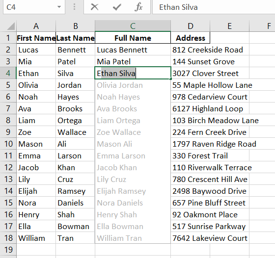
Let’s say you have a list of employees’ names divided into two columns: first and last names, and you want to combine these names into a single cell.

Instead of manually typing each first name, just do this:

1. In cell C2, type “Lucas Bennett” and press Enter.
2. In cell C3, start typing the full name.
3. As you type, Excel will recognize the pattern (you’re extracting the first word from the cell to the left) and show a grayed-out preview of all the other first names it will fill in.
4. Simply press Enter, and the entire column will be filled instantly.

That’s it! This also works for combining data, extracting middle names, formatting dates, and so much more. Flash Fill is your personal data entry assistant. You can also trigger it manually by going to the Data tab and clicking the Flash Fill button or by using the shortcut Ctrl + E.

2. Use Conditional Formatting to Make Data Stand Out

Staring at a wall of numbers can be overwhelming. How do you quickly spot the top-performing products, identify sales figures that are below target, or find duplicate entries? The answer is Conditional Formatting.

This feature allows you to automatically apply formatting such as colors, icons, or data bars to cells based on specific rules or criteria. It transforms your spreadsheet from a static table into a dynamic visual dashboard.

How it works:

Imagine you have a list of student test scores, and you want to quickly highlight any scores below 75 in red.

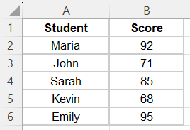
1. Select the range of cells containing the scores (B2:B6).
2. Go to the Home tab, click on Conditional Formatting, and hover over Highlight Cells Rules.
3. Choose Less Than….
4. In the dialog box, enter “75” and choose a format from the dropdown, like “Light Red Fill with Dark Red Text”.
5. Click OK.

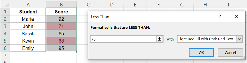
Instantly, the scores for John (71) and Kevin (68) will be highlighted. If you change a score, the formatting updates automatically. You can use this for countless scenarios: highlighting top 10% of values, color-scaling sales numbers from green to red, or adding data bars to visualize quantities.

If you are interested in reading further about this – Advanced Conditional Formatting in Excel: A Comprehensive Guide

3. Find Anything with XLOOKUP

For years, VLOOKUP was the go-to function for finding and retrieving data from a table. While powerful, it had its limitations: it could only look to the right, was prone to errors if columns were added, and had a slightly confusing syntax. XLOOKUP is the next generation that we can use for complex data sets.

XLOOKUP is simpler, more flexible, and more powerful. It can look up a value in a table and return a corresponding value from any other column, regardless of its position.

Example:

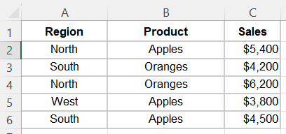
Let’s say you want to find the specific sales amount for a given Product sold in a particular Region.

=XLOOKUP(1, ($A$2:$A$6=E2) * ($B$2:$B$6=F2), $C$2:$C$6)

The formula will look for the row where the Region is “North” and the Product is “Oranges” and return the correct sales amount.

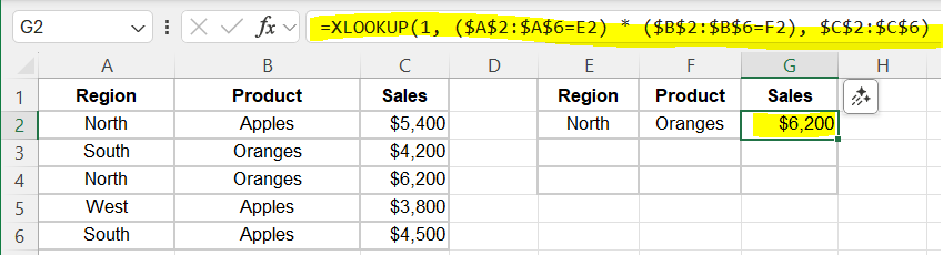
Let’s break down how the lookup_array is built. The formula has three main parts:

1. lookup_value: What we are looking for. In this case, it’s the number 1.
2. lookup_array: Where we are looking for it. This is the clever part: ($B$2:$B$6=F2) * ($C$2:$C$6=G2).
3. return_array: The range that contains the answer we want: $D$2:$D$6.

Step 1: First Logical Test (Region)

Excel first evaluates ($B$2:$B$6=F2), which checks which cells in the Region column match our criterion in F2 (“North”). This produces a virtual array of TRUE and FALSE values.

Region	Test: Is it “North”?	Result
North	TRUE
South	FALSE
North	TRUE
West	FALSE
South	FALSE

Step 2: Second Logical Test (Product)

Next, Excel evaluates ($C$2:$C$6=G2), which checks which cells in the Product column match our criterion in G2 (“Oranges”). This produces a second virtual array.

Product	Test: Is it “Oranges”?	Result
Apples	FALSE
Oranges	TRUE
Oranges	TRUE
Apples	FALSE
Apples	FALSE

Step 3: Multiplying the Arrays

This is the key step. Excel multiplies the results of the two arrays. In Excel’s calculations, TRUE = 1 and FALSE = 0. The multiplication looks like this:

Test 1 (Region)	Test 2 (Product)	Calculation	Final Array
TRUE (1)	FALSE (0)	1 * 0	0
FALSE (0)	TRUE (1)	0 * 1	0
TRUE (1)	TRUE (1)	1 * 1	1
FALSE (0)	FALSE (0)	0 * 0	0
FALSE (0)	FALSE (0)	0 * 0	0

The only way to get a 1 in the final array is if both conditions were TRUE. This final array, {0; 0; 1; 0; 0}, becomes the lookup_array.

Putting It All Together

Now the formula is simple for Excel to solve:

1. Return Array: Excel goes to the third position of the return_array ($D$2:$D$6) and returns the value it finds there, which is $6,200.
2. Lookup Value: Look for the number 1.
3. Lookup Array: Search for that 1 inside the virtual array {0; 0; 1; 0; 0}. Excel finds it in the third position.

4. Summarize Data in Seconds with PivotTables Seconds

If you work with large datasets, PivotTables are the single most powerful time-saving tool in Excel. A PivotTable is an interactive tool that allows you to quickly summarize, analyze, explore, and present your data. You can transform thousands of rows of raw data into a meaningful summary report with just a few clicks.

How it works:

Imagine you have a sales report with 1,000 rows of data, including columns for Region, Product Category, and Sales Amount. You want to see the total sales for each product category within each region. Doing this with formulas would be a nightmare. With a PivotTable, it takes less than a minute.

1. Click anywhere inside your data set.
2. Go to the Insert tab and click PivotTable. Excel will automatically select your data range. Click OK.
3. A new sheet will open with a PivotTable Fields pane on the right.
4. Now, simply drag and drop the fields:
   • Drag the Region field to the Rows area.
   • Drag the Product Category field to the Columns area.
   • Drag the Sales Amount field to the Values area.

Instantly, Excel creates a clean, summarized table showing total sales for each category, broken down by region, complete with grand totals. You can then easily “pivot” the data by dragging fields to different areas to see the information from a new perspective.

5. Navigate and Select Data Like a Pro

Stop slowly dragging your mouse to select hundreds or thousands of rows. Excel has powerful keyboard shortcuts that let you navigate and select large data ranges in the blink of an eye. The key is the Ctrl and Shift keys combined with the arrow keys.

How it works:

• Ctrl + Arrow Key: This shortcut jumps your cursor to the last cell with data in that direction before an empty cell. For example, if your cursor is in cell A1 of a large table, pressing Ctrl + ↓ will instantly take you to the last row of the table. Pressing Ctrl + → will take you to the last column.
• Ctrl + Shift + Arrow Key: This combines the navigation power of the Ctrl key with selection. Pressing Ctrl + Shift + ↓ will select all the cells from your current position down to the last cell with data in that column.

To select your entire data table in two seconds:

1. Click on the top-left cell of your data (e.g., A1).
2. Press Ctrl + Shift + → to select the entire first row.
3. While still holding Ctrl + Shift, press ↓ to extend the selection down to the bottom of the table.

Your entire dataset is now selected, ready for formatting, copying, or creating a chart.

6. Use the Quick Analysis Tool for Instant Insights

Sometimes you just need a quick chart or a simple total without the full commitment of building a PivotTable or writing formulas. The Quick Analysis Tool is perfect for this. It pops up whenever you select a range of data and offers instant access to formatting, charts, totals, tables, and sparklines.

How it works:

1. Select a range of data, for example, a list of monthly sales figures.
2. A small icon will appear at the bottom-right corner of your selection. This is the Quick Analysis Tool. Click it, or press Ctrl + Q.
3. A menu will appear with several tabs:
   • Formatting: Preview different types of conditional formatting.
   • Charts: Get recommended charts for your data, like a column or line chart.
   • Totals: Quickly add a Sum, Average, or Count to the bottom or right of your data.
   • Tables: Instantly format your data as a table or create a PivotTable.
   • Sparklines: Add mini-charts within a single cell to visualize trends.

Hover over any option to see a live preview. This tool is fantastic for exploring your data and adding professional-looking analysis with minimal effort.

7. Unlock the Power of Paste Special

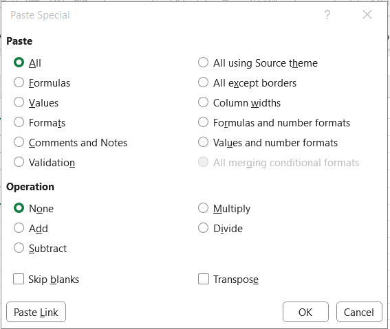
We all know Ctrl + C to copy and Ctrl + V to paste. But what if you only want to paste the calculated value of a formula, not the formula itself? Or maybe you want to copy the formatting from one cell to another without overwriting the content. That’s where Paste Special comes in.

After copying a cell (Ctrl + C), instead of just pasting, use the shortcut Ctrl + Alt + V (or right-click and choose Paste Special) to open a dialog box with a whole new world of options.

Some of the most useful options:

• Values (V): This is a lifesaver. It pastes only the result of a formula. This is perfect for freezing calculations or before deleting the source data.
• Formats (T): Copies the cell’s formatting (font, color, borders, number format) and applies it to the destination cells without changing their content.
• Column Widths (W): Pastes the column width of the copied cells. No more manually resizing columns to match!
• Transpose (E): This is incredibly useful. It switches your data from rows to columns, or vice versa.

By mastering Paste Special, you gain precise control over your data, saving you from the frustrating process of re-formatting and re-calculating.

Some Advanced Tips 

1. Named Ranges for Dynamic Navigation and Formula Writing

Have you ever struggled to write calculations like =SUM(Sheet2!A1:A500)? Every time you change data in a cell, you have to manually update the cell references. It is complex and time-consuming.

In this case, named ranges can help you a lot. Named Ranges let you assign a name to a collection of cells, for example, calling the range A1:A500 “SalesData”. Instead of writing =SUM(A1:A500), you use =SUM(SalesData), which is easier to understand, reuse, and manage.

How to Use:

• Select your cell range (e.g., A1:A500).
• Select the “Name Box” located beside the formula bar.
• Type a name like “SalesData” and hit Enter.
• Now you can use that name in formulas anywhere in your workbook.

It simplifies formula writing, makes your spreadsheet self-documenting, and improves navigation.

You can use the Name Manager (Formulas tab > Name Manager) to edit or delete named ranges.

2. Fuzzy Lookup Add-in: Match Imperfect Data

When you are working with data from many sources, such as customer records, email lists, or sales reports, names and entries frequently do not match exactly. 

For example, one page could say “Jon Smith” and another say “John Smith.” VLOOKUP and MATCH functions will not work if the values are not perfect, resulting in mismatched data or manual corrections.

So, in this case, you can use the Fuzzy Lookup Add-in (a free tool from Microsoft) to match values that are comparable rather than exact. It uses clever algorithms to determine the best approximate match.

You can install it from Microsoft’s official website. Once installed, it adds a new Fuzzy Lookup Tab to your Excel ribbon.

How to Use:

1. Prepare both data tables in your worksheet.
2. Click on the Fuzzy Lookup Tab.
3. Set the left and right tables you want to compare.
4. Choose the columns to match (like “Customer Name”).
5. Click Go, and it will return results with similarity scores, helping you match even imperfect records.

Time Saving Excel Tips: Wrap Up

Mastering Excel requires years of training, but sometimes, all it takes is learning the right Excel shortcuts and quick Excel tricks that make your daily tasks easier and faster. The tips shared in this article aren’t just random features; they’re practical Excel hacks designed to solve common data management challenges many users face.

By applying even a few of these techniques, you’ll notice a significant boost in your productivity in Excel, whether you’re cleaning data, analyzing information, or simply organizing your spreadsheets more efficiently.

So next time you open a spreadsheet, try out these time-saving tricks. You’ll be surprised at how much faster and smarter you can work, and you might even wish you had learned them sooner.