
Has it ever happened to you that when you share your spreadsheet with your colleagues or team members, important information gets lost and can’t be recovered? This is what most people face.
In this case, locking your data sheet may be the best way for you to protect your data. By locking your data sheets, others will only be able to view them and not change them.
So, in this Excel beginner’s guide, you’ll learn how to lock cells in Excel to protect Excel data sheets and cells, as well as how to unlock cells for each use.
How Excel Protection Works
In Excel, all cells are protected by default, but the lock does not take effect unless you protect your worksheet. After protecting your worksheet, you will be able to select which cells should stay editable and which should be locked. In this manner, your data sheet will be protected, and you will never lose any important information or data.
Locking a cell indicates that it is protected, whereas protecting the data sheet indicates that the lock is enabled.
After locking the cells and securing the data sheet, you can choose whether to allow users to select locked/unlocked cells, format cells, insert rows, and so on.
Lock All Cells in Excel to Protect Your Worksheet
Simply following the steps mentioned above allows you to protect your worksheet and lock certain cells, rows, and columns.
Step 1. Open Your Excel File
The first step is to open the worksheet that you want to protect. An important suggestion is to always make a copy of your data sheet before making any changes or protecting it. In this way, if you accidentally delete your data, you can recover it from a backup copy.
Step 2. Unlock All Cells (If Needed)
As previously discussed, all Excel cells are locked by default. So, if you only want to lock some specific cells, you must first unlock them. To unlock the cells, first follow the instructions mentioned below.
- Use the shortcut Ctrl + A to highlight the whole worksheet
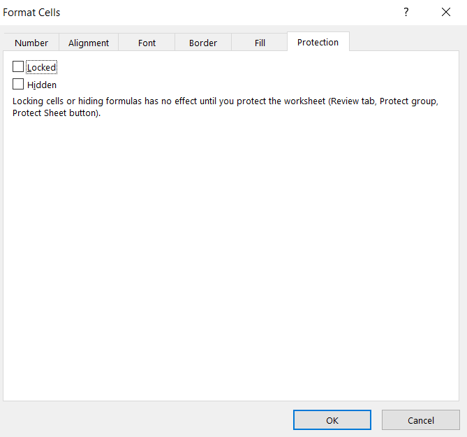
- Right-click > Format Cells.
- Go to the Protection tab.
- Uncheck Locked, then click OK.
Step 3. Select and Lock Specific Cells
After unlocking all of the cells, you have to choose the specific cells, rows, and columns that you want to protect or lock.
- Right-click > Format Cells.
- In the Protection tab, check Locked.
- Click OK.
The cells you selected will now be marked as locked in the Excel sheet.
Step 4. Protect Excel Sheet
After you’ve locked specific cells, you have to protect your worksheet.
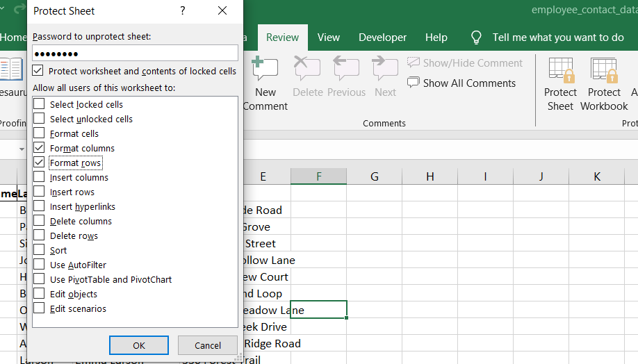
- Go to the Review tab on the ribbon.
- Click on Protect Sheet.
- A dialog box appears. You can:
- Enter a password
- Choose permissions for users (e.g., select unlocked cells, format columns)
- Click OK.
- If you entered a password, confirm it in the next dialog.
After Protection
After securing your worksheet, whenever you share it with anyone, they will only be able to view it.
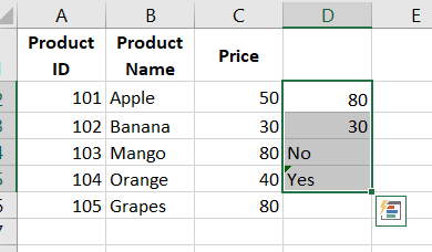
They cannot update it unless you allow them. If a user attempts to change the worksheet, a dialog box with a warning will appear in the spreadsheet, as shown below.
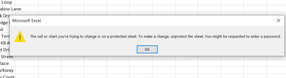
As you can see, a password is required to unlock the worksheet before it can be changed or edited. So your worksheet is completely protected now.
Lock and Hide Formula Cells
Sometimes you need to lock the formula cells, but also need to hide them from showing in the formula bar when we select these cells. So yes, it’s possible as well.
- Select the cells that contain the formulas.
- Right-click and choose Format Cells.
- Now, repeat the method we used to lock certain cells. Go to the protection tab, check Locked and Hidden, and then click OK.
- Then, go to Review > Protect Sheet, and apply sheet protection with or without a password.
Finding and Then Locking Formula Cells
If you don’t know how many cells contain formulas and want to choose all of them, you can start by selecting all of the cells and then repeat the process of unchecking the locked cells.
Go to the home tab and pick Find and select in the editing group.
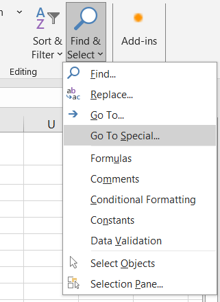
Go to special, then pick formulas, and then click OK. Excel will now select all of the formula cells. And now you can lock and hide the selected cells.
After locking the formula cells you’ve chosen, the cells will be locked from editing, and the formulas will also disappear from view in the formula bar.
The formula will not appear in the formula bar until the sheet is unprotected.
This is especially useful in financial models, templates, or reports where end users do not require formula visibility.
Password-Protected Access to Specific Cells in Excel
If you need to protect your worksheet but want to still allow certain users to edit specific parts of it, Excel makes that possible with a feature called “Allow Edit Ranges.”
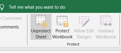
Before setting it up, make sure the sheet is unprotected. Go to the Review tab, click “Unprotect Sheet,” and enter the password if prompted.
Next, select Allow Edit Ranges from the Review tab. In the dialog box that appears, click New to define the cells or range you want others to edit.
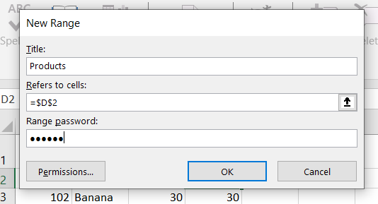
Give this range a clear name in the Title box. In the Refers to cells field, either type in the cell references or select them directly in the sheet. If you select the cells before opening the dialog, Excel will automatically fill this in for you.
To restrict access, enter a password in the Range password box. If you leave this blank, anyone can edit the range even when the sheet is protected.
Click OK and confirm the password. Once you’ve finished, protect the sheet again. Now, only users who know the range password can make changes to that section, while the rest of the sheet remains locked.
This method is a practical way to maintain control over your data while still allowing trusted users to update the information they need to work with.
Locking Entire Worksheets or Workbooks
If you want to protect the entire Excel data file or worksheet, simply skip the unlocking process that we used before protecting cells and move straight to Protect Worksheet.
If you want to secure the entire workbook, first go to Review > Protect Workbook and then select Protect Structure. Next, create a password and select OK to finish the process.
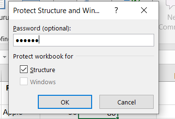
Your entire workbook is now protected, including all of the Excel data sheets and files.
Unlock Protected Sheets
To unlock the worksheet, simply click Unprotect Sheet from the Review tab, and your sheet will be unlocked. Following that, you will be able to modify cells or your worksheet.
Creating a Protected Excel File with a Password
Here’s a different method for password-protecting the entire workbook so that only authorized people can view or modify it.
Click File > Save As, choose a location.
Within the dialogue box, choose Tools and then select General Options located at the bottom right corner.
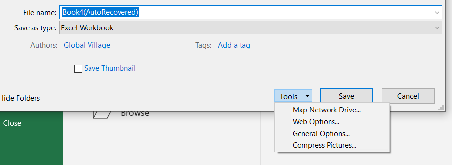
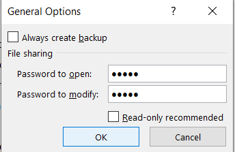
Now, set passwords, click OK, reconfirm passwords, and at last save the file.
How to Lock Cells in Excel: Wrap Up
To prevent accidental changes or data loss, it’s essential to protect your Excel sheet before sharing it. Whether you’re locking individual cells, hiding formulas, or securing the entire file, Excel gives you several flexible options to protect cells in Excel and ensure only authorized users can make edits. This guide has covered key beginner Excel how-to steps for managing protection efficiently.
Now that you know how to lock Excel data files and create a protected Excel file with passwords, you can confidently share your work without worry. By using features like “Protect Sheet” and “Allow Edit Ranges,” you maintain control over your data while still allowing limited access when needed.